Simulating Diversity Estimates
This method was described in two papers:
Brocklehurst, N. 2015. A simulation-based examination of residual diversity estimates as a method of correcting for sampling bias. Palaeontologia Electronica (18.3.7T): 1-15,
Dunhill, A., Hannisdal, B., Brocklehurst, N. & Benton, M. 2018. On formation-based sampling proxies and why they should not be used to correct the fossil record. Palaeontology (61): 119-132
See these papers for references and more detail on the concepts
When we’re studying the evolutionary history of a group, probably the most basic, fundamental thing we want to know is how many species there are in that group at different points in time. With this information we can have the background information necessary to examine crucial issues surrounding mass extinction, evolutionary radiations, competition and co-evolution. But, as in pretty much every question in palaeontology, we are hampered by the incompleteness of the fossil record.
Now, the fossil record has always been known to be incomplete; this was discussed in detail by Darwin way back in Origin of Species. But it wasn’t until the 1970s that people really began to consider that this incompleteness was not random, but in some ways systematic. It could therefore be tested, and even corrected for. David Raup, the grandfather of quantitative palaeontology, lead the way in 1972, demonstrating a strong correlation between the number of genera at any point in time, and the volume of sedimentary rock dated to those times. Are our diversity curves really showing us “diversity”, or are they simply showing us how much rock we have available to sample? Diversity estimates have also been shown to correlate with more 'human' biases, such as amount of effort to sample rocks of particular ages, or research interest in a particular group. Back in 2012, Dunhill et al. showed that sites with car parks and pubs nearby tended to be better sampled!!
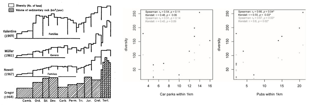
On the left, David Raup's demonstration of the correlation between rock availability and diversity estimates. Centre and right, Alex Dunhills's demonstration of the correlation between diversity estimates and availability near the sites of parking and refreshing beverages
Raup (1972) not only pioneered the concept of testing for sampling bias in the fossil record by testing for correlations between sampling proxies and diversity estimates, but also suggested that these proxies could be used to correct for the bias and produce a more reliable estimate. In short his idea was using the residuals (distance of points from the regression line between number of species and proxy) as an indication of what your diversity estimate would be if you 'removed' the signal of the proxy. This idea languished in the doldrums for a few decades, but was revived in 2007 by Smith and McGowan, and for a while became quite a popular method of assessing diversity. I used it myself in several papers, before in 2015 designing the set of simulations I'm showing here to test if it actually works.
The issue with designing a simulation to test the residual diversity estimate is that you couldn't just simulate incomplete sampling by randomly removing species. You had to simulate sampling in such a way that would also produce sampling proxies, like number of sampled formations or localities. The way I came up with was to have a clade evolve over a world with discrete regions. Species could disperse to new regions, and also go locally extinct. I could then simulate the random removal of individual species in localities (representing the taphonomic process that prevent species making it into the fossil record), random deletion of entire regions, (representing the destruction of fossil-bearing formations by geological processes), and the random deletion of fossil-bearing localities (representing the fact that palaeontologist may not have sampled that locality).
The issue with designing a simulation to test the residual diversity estimate is that you couldn't just simulate incomplete sampling by randomly removing species. You had to simulate sampling in such a way that would also produce sampling proxies, like number of sampled formations or localities. The way I came up with was to have a clade evolve over a world with discrete regions. Species could disperse to new regions, and also go locally extinct. I could then simulate the random removal of individual species in localities (representing the taphonomic process that prevent species making it into the fossil record), random deletion of entire regions, (representing the destruction of fossil-bearing formations by geological processes), and the random deletion of fossil-bearing localities (representing the fact that palaeontologist may not have sampled that locality).
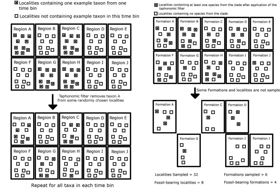
This means that you have a diversity estimate for a series of time bins drawn from an incomplete fossil record, but also sampling proxies for those time bins: number of formations sampled (the discrete regions) and number of localities sampled. These could be used to calculate a residual diversity estimate to see how well it represented true diversity. The simulation also included other methods for correcting for sampling bias, including the phylogenetic diversity estimate and (unique for this website, not included in previously published versions), John Alroy's 2018 method 'Squares'
Anyway, enough waffling now, lets get started with a tutorial on how to use the simulation code.
1. If not yet installed, install the R packages paleotree, strap and phangorn
2. Read in the three packages
library(paleotree)
library(strap)
library(phangorn)
3. Read in the diversity.sim() fuction (download via the link). The code also includes two legacy paleotree functions that have been replaced by more flexible, but much slower versions, so I prefer to use the old ones
4. Choose your analysis parameters. Lots to fiddle with here:
- local: number of fossil-bearing localities. Default 200
- form: number of formations (has to be a factor of local, as there will be the same number of localities within each formation. Default 20
- form.a: number of formations which the simulated clade will be allowed to enter. This allows you to simulate for example, that you would not expect to find a marine reptile in a terrestrial formation. Obviously has to be less than form. Default 10
-ptaph: the probability that each individual will make it through the taphonomic filter into the fossil record. Can be a number between 0 and 1, or a vector of two numbers between 0 and 1 representing the minimum and maximum probabilities. If the latter, ptaph will be drawn at random from the range each time bin. Default 0.2
- pform: the probability that each formation makes it through the geological filters. Same options and default as ptaph
- ploc: the probability that each locality will be sampled. Same options and default as ptaph.
- pmist: the proportion of nodes in the phylogeny estimated incorrectly (phylogeny used in simulating the phylogenetic diversity estimate). Number between 0 and 1. Default 0.1
- min.spec: minimum number of species in the simulated clade. Default 1000
- max.spec: maximum number of species in the simulated clade. Default 2000
- nbins: number of time bins simulated in the analysis. Default 100
- disp: probability per lineage per time bin of dispersal to a new region. Default 0.25
- ext: probability per lineage per time bin of local extinction from one occupied region. Default 0.25
5. For the purposes of this example we'll just use the default settings.
test<-diversity.sim<(local=200,form=20,form.a=10,ptaph=0.2,pform=0.2,ploc=0.2,pmist=0.1,
min.spec=1000,max.spec=2000,nbins=100,disp=0.25,ext=0.25)
test
6. The output is a matrix. Each column is a time bin, and each of there are 24 rows:
- "True Diversity": The actual number of species present in each time bin before all sampling filters
- "SIB TDE": Sample in bin taxic diversity estimate. The simplest way to estimate of diversity: count the number of species sampled in each time bin
- "RT TDE": Range through taxic diversity estimate. Again, counting the number of species sampled in each time bin, but also includes Lazarus taxa (unsampled gaps in a species range e.g. a species present in bin 1 and 3 was presumably present in bin 2)
- "PDE": Phylogenetic diversity estimate. Estimating diversity from the phylogeny by counting number of lineages in each time bin (includes ghost lineages; lineages not sampled in the fossil record but inferred from the phylogeny by working on the assumption that two sister taxa must have diverged from their common ancestor at the same time)
- "Squares": The squares equation: S + s1^2 * sum(N^2) / (sum(N)^2 - s1 * S), if N is the number of occurrences, S is the number of species, s1 is the number of singletons (species known from one occurrence). Note, some time bins may be Inf; they are the bins where all species were singletons
- "RDE Form A": Residual Diversity Estimate, calculated using number of formations bearing fossils of your clade of interest.
- "RDE Form B": Residual Diversity Estimate, calculated using number of formations bearing fossils of your clade of interest or a larger clade containing your clade of interest (this is an attempt to deal with redundancy: if a clade was in reality more diverse, you'd expect there to be more formations bearing it).
- "RDE Form C": Residual Diversity Estimate, calculated using total number of formations sampled that could have preserved fossils of your clade (i.e. where the clade was permitted to disperse) whether they bear fossils of your clade of interest or not.
- "RDE Form D": Residual Diversity Estimate, calculated using total number of formations sampled whether they bear fossils of your clade of interest or not.
- "RDE Loc A": Residual Diversity Estimate, calculated using number of localities bearing fossils of your clade of interest.
- "RDE Loc B": Residual Diversity Estimate, calculated using number of localities bearing fossils of your clade of interest or a larger clade containing your clade of interest.
- "RDE Loc C": Residual Diversity Estimate, calculated using total number of localities sampled that could have preserved fossils of your clade (i.e. where the clade was permitted to disperse) whether they bear fossils of your clade of interest or not.
- "RDE Loc D": Residual Diversity Estimate, calculated using total number of localities sampled whether they bear fossils of your clade of interest or not.
- "Proxy Form A": Sampling proxy; number of formations bearing fossils of your clade of interest.
- "Proxy Form B": Sampling proxy; number of formations bearing fossils of your clade of interest or a larger clade containing your clade of interest.
- "Proxy Form C": Sampling proxy; total number of formations sampled that could have preserved fossils of your clade (i.e. where the clade was permitted to disperse) whether they bear fossils of your clade of interest or not.
- "Proxy Form D": Sampling proxy; total number of formations sampled whether they bear fossils of your clade of interest or not.
- "Proxy Loc A": Sampling proxy; number of localities bearing fossils of your clade of interest.
- "Proxy Loc B": Sampling proxy; number of localities bearing fossils of your clade of interest or a larger clade containing your clade of interest
- "Proxy Loc C": Sampling proxy; total number of localities sampled that could have preserved fossils of your clade (i.e. where the clade was permitted to disperse) whether they bear fossils of your clade of interest or not.
- "Proxy Loc D": Sampling proxy; total number of localities sampled whether they bear fossils of your clade of interest or not.
- "pform": pform for that time bin (will only be variable if the argument was a range)
- "ploc": ploc for that time bin (will only be variable if the argument was a range)
- "ptaph": ptaph for that time bin (will only be variable if the argument was a range)
References
Brocklehurst, N. 2015. A simulation-based examination of residual diversity estimates as a method of correcting for sampling bias. Palaeontologia Electronica (18.3.7T): 1-15
Dunhill, A., Hannisdal, B., Brocklehurst, N. & Benton, M. 2018. On formation-based sampling proxies and why they should not be used to correct the fossil record. Palaeontology (61): 119-132
Dunhill, A.M., Benton, M.J., Twitchett, R.J. & Newell, A.J. 2012. Completeness of the fossil record and the validity of sampling proxies at outcrop level. Palaeontology (55):1155-1175.
Alroy, J. 2018. Limits to species richness in terrestrial communities. Ecology Letters (21): 1781-1789
Raup, D. M., 1972. Taxonomic diversity during the Phanerozoic. Science (177): 1065-1071.
Smith, A. B. and McGowan, A. J., 2007. The shape of the Phanerozoic palaeodiversity curve: how much can be predicted from the sedimentary rock record of western Europe. Palaeontology (50): 765-774.
