Analysis of Evolutionary Constraint
This method was described in Brocklehurst, N., Panciroli, E., Benevento, G. L., & Benson, R. B. J. 2021. Mammaliaform extinctions as a driver of the morphological radiation of Cenozoic mammals. Current Biology (In Press). See this paper for references and more detail on the concepts.
Understanding why some groups are more diverse, whether in terms of number of species or variety of morphologies, is one of the key questions for palaeontologists and evolutionary biologists. GG Simpson's concept of the adaptive radiation has dominated discussion of this issue since the 40s; the idea is that ecological opportunity, created when some species die out and leave niches vacant or when a key innovation allows a group to enter new niches, leads to massive increases in morphological diversity.
Adaptive radiations of morphology have usually been discussed in terms of rates: how fast has a lineage evolved. However, constraint, that is how many different traits is a lineage able to evolve, is relatively unexplored. This despite the fact that constraints are extremely important in morphological diversification. Ultimately a lineage can evolve as fast as it likes, but if its constrained to just a few areas of morphospace it's not going to get any more diverse.
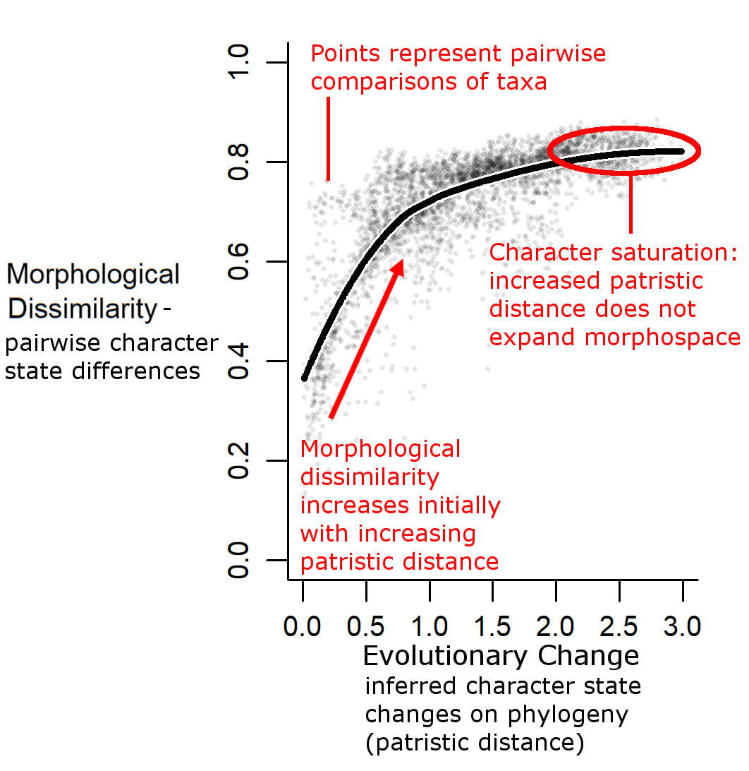
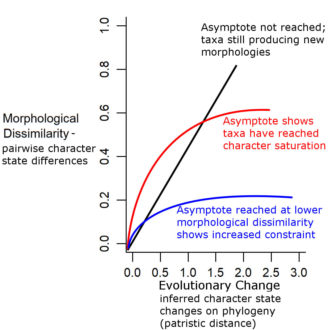
The method here allows us to test constraints on a particular group of organisms, using matrices of discrete characters. The method uses the concept of character saturation, or exhaustion: the point at which evolution stops producing new morphologies and starts producing the same few morphologies over and over again. Lets say you have a graph. Along the horizontal axis is amount of evolutionary change, up the vertical axis is morphological diversity. As the former increases, you expect the latter to increase, producing a linear relationship. As we reach the point of character saturation, however, the line starts to asymptote: further increases along the horizontal produce no further increases on the vertical. This is the point of character saturation. The lower the morphological diversity at the point of character saturation, the stronger the evolutionary constraints. In the method being discussed here, we use pairwise comparisons of taxa: the patristic distance between pairs of taxa (the number of character state changes that have occurred since their divergence) represents the amount of evolution (horizontal axis); the morphological distance between pairs of taxa (proportion of character state differences between them) represents the morphological diversity (vertical axis).
In the original paper describing the method and applying it to mammals, I provided a script in the supplementary data to allow replication of the analysis. However the script is pretty specific; it won't really help you if you want to analyse your own dataset. So here I provide the essence of the script , distilled into three functions, which should work on any dataset you care to throw at it. So, here's how to use it
1. If not yet installed, install the packages Claddis*, adephylo, and drc
*NOTE: the version of Claddis needs to be at least version 0.6.3 as older versions have different formatting for functions used in the analyses here
2. Read in these packages
library(Claddis)
library(adephylo)
library(drc)
3. Download and read in the three functions.
4. Download the example files. You will need: a character taxon matrix in nexus form (this one is the same one from Zhou et al. 2019 that was used in our original study), a tree in nexus form where branch lengths are scaled to character change on them (this one is from a Bayesian analysis of the matrix) and a csv file with the groups to be compared. This should be two columns: the first with the taxa of interest (does not need to include every taxon in the tree) and the second the group it is placed in**. Pit these in your working directory; you can check what your working directory is with the line:
getwd()
**NOTE: the groups can be anything. Clade, diet, time...for the example these are divided into non-theria (1), stem theria (2) and crown theria (3)
5. Load the matrix and store as an object called "matrix".*** Load the tree and store as an object called "tree". Load the groups and store as an object called "group". Then drop any taxa from the tree that are not included in the "group" file (these are those that are not of interest to our study)
matrix<-read_nexus_matrix("matrix.nex")
tree<-read.nexus("tree.tre")
group<-read.csv("group.csv",header=T)
tree<-drop.tip(tree,which(tree$tip.label%in%group[,1]==F))
***NOTE: The function read_nexus_matrix() from Claddis can be a bit fussy over the formatting of the nexus file. Make sure there are no spaces and that there is an assumption block
6. First we will calculate patristic distances. This will produce a pairwise distance matrix, giving the distance between all possible pairs of taxa.
pat.dist<-as.matrix(distTips(tree,method = "patristic"))
7. Next we will calculate the morphological distances between taxa. For this example I'm using the MORD distance metric. Then we will again remove any taxa that are not of interest.
dist<-calculate_morphological_distances(matrix, distance_metric = "mord",distance_transformation= "none")
morph.dist<-dist[[2]]
morph.dist<-morph.dist[rownames(pat.dist),rownames(pat.dist)]
8. Use the new find.pairs() function to identify and categorise all possible pairwise combinations of taxa. It has three arguments.
- groups: an object of class "matrix" with two columns containing the taxa under study and the group they are assigned to
- morph.dist: an object of class "matrix", containing pairwise morphological distances between all taxa.
- pat.dist: an object of class "matrix", containing pairwise patristic distances between all taxa.
It produces a matrix where each row represents a pairwise comparison of two taxa, with six columns . "Taxon 1" and "Taxon 2" are the taxon names. "Group 1" and "Group 2" are the groups to which each taxon is assigned to. "Morphological distance" and "Patristic distance" are the two distances between them.
pairs<-find.pairs(group,morph.dist,pat.dist)
9. To plot the curves to illustrate constraint, use the new function plot.groups(). This contains four arguments, as well as the abbility to use all the usual arguments from par()
- data: an object of class "matrix", containing the output from the find.pairs() function
- col.point: an object of class "list", containing as many items as there are groups. Each item in the list will be a colour or rgb() function determining the colour assigned to the points representing pairs of taxa in each group
- col.line: an object of class "list", containing as many items as there are groups. Each item in the list will be a colour or rgb() function determining the colour assigned to the lines representing loess fitted regression curves of the points in each group
- lwd.shadow=NULL: an object of class numeric. Represents the thickness of a white line behind each loess curve; if this is thicker than the thickess of the line itself (represented by the usual lwd parameter), then this can make the line stand out more.
A legend may be added in the usual way using the legend() function
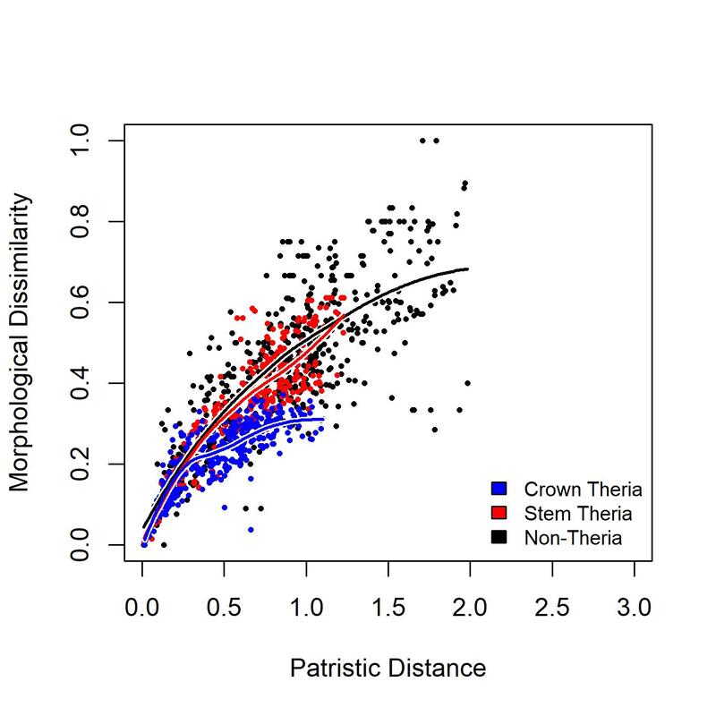
plot.groups(data=pairs,col.point=list("black","red","blue"),col.line=list("black","red","blue"),lwd.shadow=4,pch=16,lwd=2,cex=0.5)
legend("bottomright",legend=c("Crown Theria","Stem Theria","Non-Theria"),fill=c("Blue","Red","Black"),bty="n",cex=0.8)
So, from this graph we can see that Crown therians and non-therians have reached character saturation: their curves have reached asymptote, so further evolution is not producing new morphologies. Crown therians reached asymptote at a lower morphological distance than non-therians; they are under greater constraint. Stem therians have not yet reached the limits of their constraint; their curve has not reached asymptote, so they are still exploring new morphologies.
10. Finally, we want to see if our groups are significantly constrained or under significantly relaxed constraints. The new function char.sat() will first infer the morphological distance at character saturation for each group, by fitting a Michaelis-Menten curve to the data and using the Vmax parameter as an estimate of the point of character saturation. Then null character matrices are simulated under equal rates models, and the pairwise comparisons are carried on these matrices as described above. You can then compare the null values from each group to the observed values. The function char.sat() has four arguments:
- tree: an object of class "phylo". The tree with branch lengths scaled to number of character changes
- matrix: a character matrix imported using read_nexus_matrix()
- data: an object of class "matrix", containing the output from the find.pairs() function
- group: an object of class "matrix" with two columns containing the taxa under study and the group they are assigned to (as in the find.pairs() function above)
- nsim: an object of class "numeric". The number of null simulations to be carried out
- metric: an object of class "character" indicating what morphological distance metric to be used in the null simulations (options the same as those in the calculate_morphological_distances function in Claddis)
The function outputs a list of length two. The first item in the list is a vector containing the inferred point of character saturation in each group. The second contains a matrix with each row representing a null simulation and each column representing a group, containing the null saturation points for each group. These can be compared to the observed values; if the observed values are higher than the null expectations, the group is under significantly relaxed constraint. If the observed values are lower the group is under significantly higher constraint.
signif<-char.sat(tree,matrix,pairs,group,100,"mord")
signif[[1]]
signif[[2]]
signif<-char.sat(tree,matrix,pairs,group,100,"mord")
signif[[1]]
signif[[2]]


